Lecture: 17 - 18

[ Home ][ PDF ]

Topics: Linearized polynomials, Feedback Shift registers

Linearized polynomials

Chapter 3, 3-4

Linearized polynomials are among the most importatnt types of polynomials which have many applications. The trace function are among these.

A useful feature of these polynomials is the structure of the set of roots that facilitates the determination of the roots.

Let $q$ denote a prime power, for this section.

Theorem 3.11 Determening the order

Let $\mathbb{F_{q}}$ be a finite field of characteristic $p$, and leg $f\in \mathbb{F_q}[x]$ be a polynomial of positive degree and with $f(0) \neq 0$. Let $f = a \cdot f_{1}^{b_1} \dots f_{k}^{b_k} $ where $a \in \mathbb{F_{q}}, b_1 \dots b_k \in \mathbb{N}$ and $f_1 \dots f_k$ are distinct monic irreducible polynomials in $\mathbb{F}{q}[x]$, be the canonical (relating to) factorization of $f$ in $\mathbb{F}{q}[x]$. Then $ord(f) = e\cdot p^t$ , where $e$ is the least common multiple of $ord(f_1), \dots , ord(f_k)$ and $t$ is the samlles integer with $p^t \geq max(b_1, \dots, b_k)$.

A method of determining the order or an irreducible polynomial $f$ in $\mathbb{F}_{q}[x]$ with $f(0) \neq 0$ is based on the observation that the order $e$ of $f$ is the least positive integer s.t $x^e \equiv 1 \mod f(x)$.

Furthermore, by collaray 3.4, $e$ divides $q^m-1$ , where $m = deg(f)$. Assuming $q^4 \gt 2$, we start from the prime factor decomposition.

$$q^m - 1 = \prod_{j = 1}^{s} p_{j}^{r_{j}}$$

For $1 \leq j \leq s$ we calculate the residues of $x^{(q^m-1)/p_j} \mod f(x)$. This is accomplished by multiplying together a suitable combination of the residues of $x,x^q, x^{q^2}, \dots , x^{q^{m-1}}$ mod $f(x)$.

If $x^{(q^m-1)/p_j} \not\equiv 1 $ mod $f(x)$, then $e$ is a multiple of $p_{j}^{r_{j}}$. In the latter case we check to see wheter $e$ is a multiple of $p_{j}^{r_{j}-1}, p_{j}^{r_{j}-2}, p_j$ by calculating the residues of

$$x^{(q^m-1)/p_j^2}, x^{(q^m-1)/p_j^3}, \dots , x^{(q^m-1)/p_j^{r_j}} \mod f(x)$$

This computation is repeated for each prime factor of $q^m-1$. A key step in the method above is the factoriztion of the ingeter $q^m-1$. There exist extensive tables for the complete factorization of numbers of this form, especially for the case $q = 2$.

3.12 Definition of Reciprocal polynolial

Let $f(x)$ with $a_n \neq 0$ be defined as follows: $f(x) = a_n\cdot x^n + a_{n-1} \cdot x^{n-1} + \dots + a_1 \cdot x + a_0 \in \mathbb{F}_{q}[x]$

Then the reciprocal polynomial $f^*$ of $f$ is defined by:

$$f^*(x) = x^n \cdot f \bigg(\frac{1}{x}\bigg) = a_0 \cdot x^n + a_1 \cdot x^{n-1} + \dots + a_{n-1} \cdot x + a_n$$

Definition $q$-polynomial

A polynomial of the form:

$$L(x) = \sum_{i=0}^{n}\alpha_i \cdot x^{q^i}$$

with coefficients in an extension field $\mathbb{F_{q^{m}}}$ of $\mathbb{F}{q}$ is called a $q$-polynomial over $\mathbb{F}{q^m}$

If the values of $q$ is fixed once and for all or is clear from the context, it is also cutomary to speak of a lineariezed polynomial. If $F$ is an arbitraty extension field of $\mathbb{F}{q^m}$ and $L(x)$ is a linearized polynomial over $\mathbb{F}{q^m}$ then:

$$L(\beta + \gamma ) = L(\beta) + L(\gamma) , \forall \beta, \gamma \in F$$ $$L(c\cdot \beta ) = c \cdot L(\beta), \forall c \in \mathbb{F}_{q}, \forall \beta \in F$$

The identity (3.11) follows immediatly from Theorem 1.46 and (3.12) follows from the fact that $c^{q^i} = c$ for $c \in \mathbb{F}{q}$ and $i \geq 0$. If $F$ is considered as a vectorspace over $\mathbb{F}{q}$ then the linearized polynomial $L(X)$ induceds a linear operator on $F$.

This is shown in 3.50.

Theorem 3.50 Roots form a linear subspace

Let $L(X)$ be a nonzero $q$-polynomial over $\mathbb{F_{q^{m}}}$ and let the extension field $\mathbb{F}{q^s}$ (notice that s) over $\mathbb{F}{q^m}$ contain all the roots of $L(X)$. Then each root of $L(X)$ has the same multiplicity, which is either $1$ or a power of $q$, and the roots form a linear subspace of $\mathbb{F}{q^s}$, where $\mathbb{F}{q^s}$ is regarded as a vector space over $\mathbb{F}_{q}$

The proof follows from 3.11 and 3.12 that any linear combination of roots with coefficients in $\mathbb{F}{q}$ is again a root, and so the roots of $L(x)$ form a linear subspace of $\mathbb{F}{q^s}$.

Proof is on page 99 of the book.

3.54 Affine $q$-polynomial

A polynomilal of the form $A(x) = L(x) - \alpha$, where $L(X)$ is a $q$-polynomial over $\mathbb{F}{q^m}$ and $\alpha \in \mathbb{F}{q^m}$, it is called an affine $q$-polynomial over $\mathbb{F}_{q^m}$

An element $\beta \in F$ is a root of $A(x)$ iff $L(\beta) = \alpha $. From 3.15, the equation $L(\beta) = \alpha$ is equivelant to:

$$(c_1, \dots , c_s)\cdot B = (d_1, \dots , d_s)$$

where $\alpha = \sum_{k=1}^{s} d_k \cdot \beta_k $.

The system of linear equations is solved for $c_1, \dots, c_s$ and each solution vector ($c_1, \dots, c_s$) yeilds a root $\beta = \sum_{j=1}^{s} c_j \cdot \beta_j$ of $A(x)$ in $F$.

The fact that roots are easier to determine for affice polynomials suggest the following method of finding roots of an arbitraty polynomial $f(x)$ over $\mathbb{F}{q^m}$ of positive degree in an extension field $F$ of $\mathbb{F}{q^m}$ .

First, determine a nonzero affine $q$-polynomial $A(x)$ over $\mathbb{F}_{q^m}$ that is divisible by $f(x)$, that is a so-called affine multiple of $f(x)$.

Next, obtain all the roots of $A(x)$ in $F$ by the method described in first point. Since the roots of $f(x)$ in $F$ must be among the roots of $A(x)$ in $F$, it suffices the to calculate $f(\beta)$ for all roots $\beta$ of $A(x)$ in $F$ in order to locate the roots of $f(x)$ in $F$.

The only point that remains to be settled is how to determine an affine multiple $A(x)$ of $f(x)$.

This can be achived as follows:

Let $n \geq 1$ be the degree of $f(x)$. For $i = 0, 1, \dots, n-1 $ calculate the unique polynomial $r_i(x)$ of degree $\leq n-1$ with $x^{q^i} \equiv r_i(x) \mod f(x)$.

Then determine element $\alpha_i \in \mathbb{F}{q^m}$, not all 0, s.t $\sum{i=0}^{n-1} \alpha_i \cdot r_i(x)$ is a constant polynomial.

This involves $n-1$ conditions converning the vanishing of the coefficients of $x^j, 1 \leq j \leq n-1$, and leads to a homogenous system of $n-1$ linear equations for the $n$ unknows $\alpha_0, \alpha_1, \dots , \alpha_{n-1}$.

A homogenous system always has a nontrivial solution. Once the nontrivial solution has been fixed, we have $\sum_{i=0}^{n-1} \alpha_i \cdot r_i(x) = \alpha $ for some $\alpha \in \mathbb{F}_{q^m}$.

It follows that

$$\sum_{i=0}^{n-1} \alpha_i \cdot x^{q^i} \equiv \sum_{i=0}^{n-1} \alpha_i \cdot r_i(x) \equiv \alpha \mod f(x)$$

and so

$$A(x) = \sum_{i=0}^{n-1} \alpha_i \cdot x^{q^i} - \alpha$$

$A(x)$ is a non affine $q$-polynomial $\mathbb{F}_{q^m}$ divisible by $f(x)$ We may take $A(x)$ to be a monic polynomial.

3.56 Roots of $A(x)$

Let $A(x)$ be an affine $q$-polynomial over $\mathbb{F}{q^m}$ of positive degree and let the extension field $\mathbb{F}{q^s}$ of $\mathbb{F}{q^m}$ contain all the roots of $A(x)$. Then each root of $A(x)$ has the same multiplicity, which is either is $1$ or a power of $q$, and the roots for an affine subspace of $\mathbb{F}{q^s}$, where $\mathbb{F}{q^s}$ is regarded as a vector space over $\mathbb{F}{q}$ Same as 3.50.

Examples of $q$-polynomials:

• $x^8$ is a $2$-polynomial over $\mathbb{F_{2^m}}$ for any positive integer $m$; it is also an $8$-polynomial over $\mathbb{F_{2^{3k}}}$ for any positive integer $k$. It has only one roort $0$ with multiplicity $8$.

• $x^8 + x$ is a $2$-polynomial over $\mathbb{F_{2^m}}$ for any positive integer $m$; it is also an $8$-polynomial over $\mathbb{F_{2^{3k}}}$ for any positive integer $k$. It has 8 different roots in $\mathbb{F_{2^{3k}}}$ which are all elements of $\mathbb{F_8}$ (Ref: Lemma 2.3 and 2.4)

• $Tr_{\mathbb{F_{16}}/\mathbb{F_2}}(x) = x + x^2 + x^4 + x^8$ is a $2$-polynomial over $\mathbb{F_{16}}$ which has 8 different roots. Since $Tr_{\mathbb{F_{16}}/\mathbb{F_2}}(x)$ can take only values in $\mathbb{F_2}$ and has degree 8, so $Tr_{\mathbb{F_{16}}/\mathbb{F_2}}(x)$ has 8 roots as well as $Tr_{\mathbb{F_{16}}/\mathbb{F_2}}(x)+1$

• $Tr_{\mathbb{F_{16}}/\mathbb{F_4}}(x) = x + x^4$ is a $4$-polynomila over $\mathbb{F_{16}}$ which has 4 different roots.

Feedback shift registers

Chapter 8, 1

Sequcens in finite fileds whose terms depend in a simple manner on their predecessors are of importance for a variety of applications. Such sequnces are easy to generate by recursive procedures, which is certainly an advantageous feature from the computational viewpoint, and they also tent to have useful structural properties.

Of particular interes is the case where the terms depend linearly on a fixed number of predecessors, resulting in a so-called linear recurring sequence.

$k$-th order

Definitions of $k$-th order linear recurring sequences in $\mathbb{F}_{q}$;

• $k$-th order linear recurrance relasion
• homogeneous and inhomogeneous relations
• inital values of a sequence.

Let $k$ be a positive integer, and leg $a, a_0, \dots, a_{k-1}$ be given elements of a finite field $\mathbb{F}{q}$. A sequence $s_0, s_1, \dots$ of elements of $\mathbb{F}{q}$ satisfying the relation

$$s_{n+k} = a_{k-1}\cdot s_{n+k-1} + a_{k-2}\cdot s_{n+k-2} + \dots + a_0\cdots s_n + a$$

for $n = 0,1,\dots$

is called a $k$-th order linear recurring sequence in $\mathbb{F}_{q}$.

The terms $s_0, s_1, \dots, s_{k-1}$, which determine the rest of the sequence uniquely, are reffered to as the inital values.

A relation of the form above is called $k$-th order linear recurrence relation. Itmay also be called “difference equation”.

We speak of homogeneous linear recurrence relation if $a=0$, otherwise it is inhomogeneous linear recurring sequence in $\mathbb{F}_{q}$.

Feedback shift register

The generation of linear recurring sequences can be implemented on a feedback shift register. This is a special kind of electronic switching circuit handling information in the form of elements of $\mathbb{F}_{q}$, which are represented suitably.

Definitions of the four types of devides used in feedback shift register:

• Adder
• Constant multiplier
• Constant adder
• Delay element

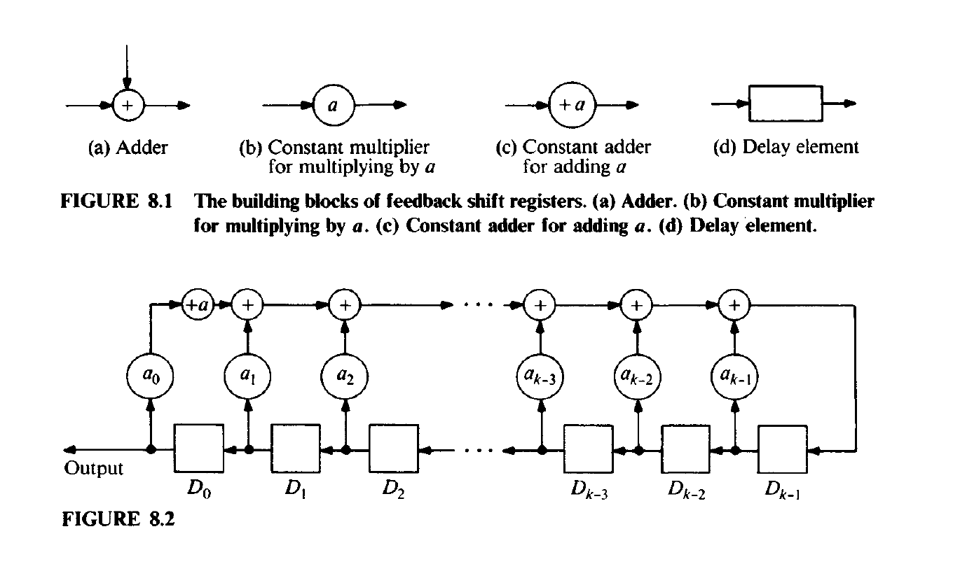Figure is from the book at page 396 or 197 old book.

The first is the adder, which has two inputs and one output, the output being the sum in $\mathbb{F}_{q}$ of the two inputs.

The second is the constant multiplier, which has one input and results in the output of the product of the input with a constant element of $\mathbb{F}_{q}$ (This just says it multiplies it).

The third is a constant adder, whiuch is analogous to a constant multiplier, but adds a constatn element of $\mathbb{F}_{q}$ to the input.

The fourth type of device is a delay element e.g “flip-flop”, which has one input and one output and is requlated by and external synchronous clock so that its input at a particular tinme appears as its output one unit of time later.

A feeback shift register is built by interconnecting a finite number of adders, constant multipliers, constant adders, and delay elements along a closed loop in such at way taht two outputs are never connected together. Actually, for the purpose of generating linear recurring sequences, it suffices to connect the componentes in a rather special manner. A feedback shift register that generates a linear recurring sequence satisfying is show in this figure.

At the outset, each delay element $D_j, j= 0,1,\dots , k-1$ contains the initial value $s_j$ If we think of aritmethic operations and the transfer alon the wires to be performed instataneously, then after one time unit each $D_j$ will contain $s_{j+1}$. Continuing in this manner, we see that theoutput of the feedback shift register is the string of elemkent $s_0, s_1, s_2, \dots $ received in intervals of one time unit. In most of the applications the desired liear recurring sequence is homogeneous, in whiche case the constant adder is not needed.

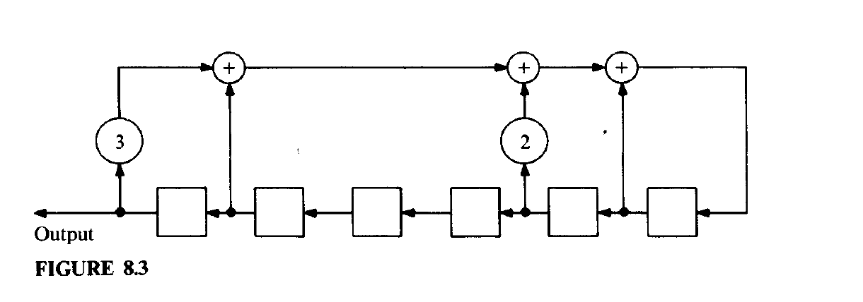
Example 1

In order to generate a linear recurring sequnce in $\mathbb{F_5}$ satisfying the homogeneous linear recurrance relation:

$$s_{n+6} = s_{n+5} + 2\cdot s_{n+4} + s_{n+1} + 3\cdot s_{n}$$

for $n = 0, 1, \dots ,$

Since $a_2 = a_3 = 0$, no connections are necessary at these points, one may use the following feedback shift register.

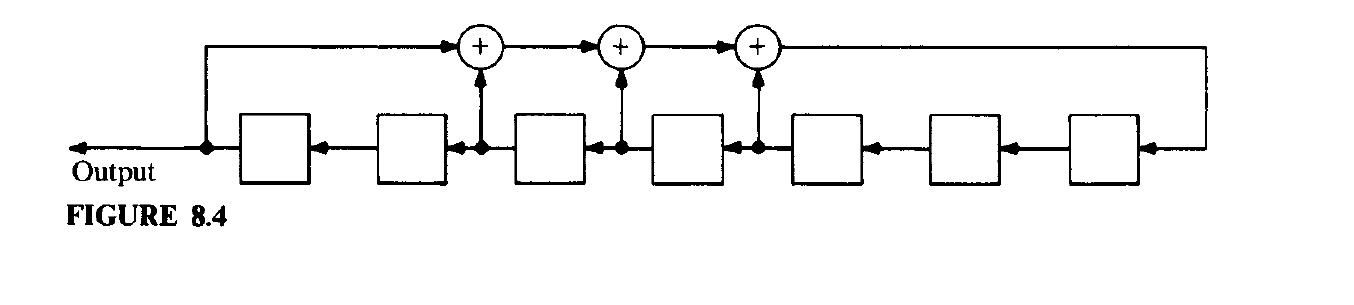
Example 2

Consider the homogeneous linear recurrence relation:

$$s_{n+7} = s_{n+4} + s_{n+3} + s_{n+2} + s_{n}, n = 0,1,\dots , \in \mathbb{F_2}$$

Since multiplication by a constant in $\mathbb{F_2}$ either preserves or annihilates elements, the effect of a constatnt multiplier can be simulated by a wire connection or a disconnection. Therefore, a feedback shift register for the generation of binary homogeneous linear recurring sequences requires only delay elements, adders and wire connections. $\square$

Figure for above example:

Let $s_0, s_1, \dots $ be a $k$-th order linear recurring sequence in $\mathbb{F}_{q}$ satisyfing:

$$s_{n+k} = a_{k-1}\cdot s_{n+k-1} + a_{k-2}\cdot s_{n+k-2} + \dots + a_0\cdots s_n + a$$

for $n = 0,1,\dots$.

This sequence can be generated by the feedback shift register in Example 1. If $n$ is a nonnegative integer, then after $n$ time units the delay element $D_j, j = 0,1,\dots, k-1$ will contain $s_{n+j}$.

It is therefore natural to call the vector $\vec{s_n} = \big( s_n, s_{n+1}, \dots, s_{n+k-1}\big)^T$ (row vector) the $n$-th state vector of the linear recurring sequence (or of the feedback shift register). The state vector $\vec{s_0} = \big( s_0, s_{1}, \dots, s_{k-1}\big)^T$ is referred to as the initial state vector.

Is is a characteristic feature of linear recurring sequences in finite fields that, after a possibly irregular behaviou in the beginning, such sequences are eventually of a periodic nature.¢¢¢